## dataset-design-and-temporal-concurrency
Welcome back!
Before getting started, let’s revisit out problem statement from the introduction:
"I want to know trends related to total cost of care; inpatient average lengths of stay; lapses in medication adherence; and member counts for the period between January first of 2019 and the end of 2020. Med lapses should show monthly totals and cumulative monthly totals. Pull members between 30 and 50 years old and have had at least two inpatient visits within a six-week period. I need to see results by month; all services received and corresponding facilities; and member demographics."
The conventions I’ll use are also defined in the introduction here.
When
Identifying the global temporal window ( \(W\) ) is important as defines the frame of reference within which temporal relations are queried and transformed. It is the absolute governor of detecting when things take place. In this case, the window is defined as all records having temporal columns or derived temporal measurements with at least one value falling within the period 2019-01-01 to 2020-12-31:
\(\forall W, D^λ \Rightarrow D^\lambda_\Omega:= \Bigg\{\matrix{ W_\text{start} \le \delta^T \le W_\text{end},\enspace\enspace\#\delta^T= 1\\ \\ W_\text{start} \le \delta^T_\text{end} \wedge W_\text{end} \ge \delta^T_\text{start},\enspace\enspace\#\delta^T= 2 }\Bigg\}\)
, where \(D^\lambda\) is the data source for context \(\lambda\) (i.e., demographics, claims, prescriptions) and \(W\) the lower and upper dates of the global window. The first form of \(D^\lambda\) above reflects the case of a single time column in \(D\) and the second form when there are two.
-
It allows for a much more compact dataset. I recommend giving serious consideration to transforming the single-date form into the dual-date form, especially when most of
\(\delta^I\)is duplicative along\(\delta^T\)(more on this in a future article) -
It allows for
\(\delta^T\)to extend outside of the bounds of\(W\)while preserving the ability to detect temporal concurrency relative to\(W\) -
Do not use the following logic to detect concurrency of the dual-date form with
\(W\)(or any other dual-date range):\((W_\text{start} \le \delta_\text{start} \le W_\text{end} ) \vee (W_\text{start} \le \delta_\text{end} \le W_\text{end})\)This logical statement will fail to capture cases where\(\delta^T\)extends outside of\(W\):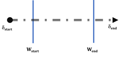
Who
The “Who” aspect of the problem statement consists of two detectable conditions (as indicated by the conjunction “and”) and a possible, third:
-
\(\omega_1\): “… members between 30 and 50 years old” -
\(\omega_2\): “… have had at least two inpatient visits within a six-week period” -
\(\omega_3\):\(f(\omega_1, \omega_2)\)— dependence vs. independence
Age vs. Report Window (\(\omega_1\))
\(\omega_1\) is the first opportunity to greatly trim down your data pull.
\(\omega_1\)must qualified relative to\(W\)and not “as of today”. Granted: this is not explicitly stated, but think about it: “… for the period between January first of 2019 and the end of 2020” is your cue. Of course, when in doubt, check with the requester just to be sure.\(W\)covers two years which will result in two ages for each member not filtered out. Question: Which age should be returned at this point? My preference would be neither and instead return the dates of birth. Age is a derived measure and is only needed to qualify records at this point; dates of birth are the temporal attributes (\(\delta^T\)) which should carried forward (I’ll explain why later).
✨ At this stage, we’ve defined the first portion of “Who” is related to the problem statement. An advantage of starting in this manner is that a maximally large cohort has been defined and can be stored in a table to which subsequent data can more efficiently be joined.
For the sake of demonstration, assume the existence of a member demographics table \((M)\). Satisfying \(\omega_1\) results in our first dataset: \(D^M:=\sigma_{\omega_1}(M)\)
, where \(\sigma\) represents a selection operation.
 Take a Break!
Events vs. Report Window (\(\omega_2\))
Now, we move on to defining (\(\omega_2\)). Assume a claims dataset \((L)\) containing multiple service types \((\delta^G: \text{Inpt}\in G)\). To satisfy this requirement, three conditionals need to be addressed:
\(c_1:= W_\text{start} \le \dot{\delta^T} \le{W}_\text{end}; \enspace\dot{\delta^T}\equiv\text{service date}\)
If dataset \(L\) has well-defined indicators for admissions (and discharges), detecting distinct events is easy. For the sake of this scenario, I will assume this to be the case [scenarios where the beginning and ending of a series are not well-defined will be covered in a separate article — eventually]:
\(c_2:=\#\big(\dot{\delta^T|}c_1\big) > 1;\enspace\dot{\delta^T}\equiv\text{admission date}\)
\(c_3:=\big({\Delta_n}\dot{\delta^T}|{c_2}\big)\ge\text{42 days}\\{\Delta_n}\dot{\delta^T}:={\dot{\delta^T}}_{i+1}-{\dot{\delta^T}}_i\Big|_{i=1}^{n-1},\enspace\text{ the time between successive admissions}\)
1st \(c_1\): This is the most restrictive and is easily accomplished with a join operation over relations \(M\) and \(S\): \(M \bowtie_{\theta \rightarrow \delta^I}{S}, \enspace\delta^I\equiv\text{member identifier}\)
2nd \(c_3\): Resolving \(c_3\) gives you \(c_2\) for free (I’ll leave that as “thought homework” for you to ponder)
3rd \(c_2\): This is easily resolved by counting over \(c_3\) and qualifying based on the prescribed threshold
The second and third steps can easily be flipped depending on the number of TRUE cases at each step. Use your domain knowledge (or someone else’s) in these cases or, if all else fails, use multiple trial-and-error runs on sampled data (sampling at the member level, in this case) to get a sense of which order will have the best performance on the full set of observations.
]{toggleGroup=4 context=“posthoc” style=“display:block”}

Temporal Dependence vs. Independence (\(\omega_3\))
In this final portion of the article, I want to offer a consideration related to the problem statement that I recommend verifying at the beginning of the data retrieval and wrangling process: temporal dependence vs. independence. Conceptually similar to (in)dependence of variables, this is in a semantic context often encountered when there is ambiguity regarding the relationships among temporal criteria that cannot simply be inferred.
For example, consider two scenarios in which \(\omega_{1}\) and \(\omega_{2}\) can be understood:
-
Scenario 1: Independence (
\(\forall W:\omega_1 \wedge\omega_2\))In this scenario,
\(\omega_1\)is sufficient, and the age calculated when resolving this criterion can be carried forward. -
Scenario 2: Dependence (
\(\forall W: \big(\omega_1|\omega_2\big)\))In this scenario, a determination (made by the requester) must be made as to which qualifying event in
\(\omega_{2}\)— first or second — serves as the point of reference to evaluate\(\omega_{1}\). Scenarios like this are why I recommended only carrying forward essential information (in this case, the member dates of birth) instead of contingent information (e.g., member age relative to\(W\)).
Problem statements related to workflows with multiple decision points frequently cause the second scenario to arise in analytic initiatives, so it is good to look into the real-world context of a request in addition to the available data.
🎉Congratulations!
You’ve made it to the end! I’ll summarize our journey so far:
-
We saw how a plain-language statement can be decomposed into smaller, logical chunks to be stepped through and interrogated.
-
We looked at the “When” and “Who” of our problem statement and explored temporally-based considerations such as global windows of time, relative time between events, and relative event sequencing.
-
We considered how the order in which criteria are addressed relates to query and processing performance.
-
I hope you see that as we work through the full statement, what emerges is a “design map” of sorts (which also helps with data product documentation).
That’s all for now — I look forward to seeing you in Part 2 where we explore the “What” of our problem statement.
Until next time, I wish you much success in your journey as a data practitioner!